Writing Your Controller¶

Each participant must implement their control algorithm in a Python file (by default, my_controller.py). This file defines the control strategy executed by the WAPPAC simulator.

The controller’s goal is to maximize the performance index \(\mathcal{G}\) over the scoring interval \(t \in [T_0, t_{end}]\) by defining the control force \(F_{pto}(t)\) appropriately for all three sea-state scenarios:

\[\max_{F_{pto}(t)} \; \mathcal{G}\!\left(F_{pto}(t); t \in [T_0,t_{end}] \right) = \frac{\bar{P}_{pto}} {2 + \frac{\left[|x(t)|\right]_{98}}{x_{\max}} + \frac{\left[|F_{pto}(t)|\right]_{98}}{F_{u,\max}} - \frac{\bar{P}_{pto}}{\left[p_{pto}(t)\right]_{98}}}\]

\[\begin{split}\text{s.t.}& \quad \text{WavePiston dynamics,} \quad \\ & \quad p_{pto}(t) = F_{pto}(t) \dot{x}(t) \ge 0 \quad \forall t \in [t_{init},t_{end}]\end{split}\]

For more details, see Control Problem Definition.

Controller Function Interface¶

Your controller must define the following function:

def my_controller(x, v, t, eta10):
    # Your control logic here defining F_pto for the current time-step
    return F_pto

Note

You may rename the Python file differently, but the function name must remain my_controller.

Function Arguments¶

Variable	Type	Description
`x`	float	Sail position [m]
`v`	float	Sail velocity [m/s]
`t`	float	Current simulation time [s]
`eta10`	float	10 m up-wave surface elevation [m] (measured at \(x=-10\) m)

Function Output¶

Variable	Type	Description
`F_pto`	float	Control force [N] applied by the PTO system

Using External Packages¶

Participants may include custom or third-party Python packages by placing them in the dedicated folder:

WAPPAC_distribution/
├── my_controller.py
├── external_packages/
│   └── [your custom packages here]

Important: The folder name must remain exactly external_packages/. WAPPAC automatically searches this directory at runtime to make its contents importable by your controller.

Installing a Custom Package Locally¶

You can install a package directly into the external_packages folder:

python -m pip install --target ./external_packages control

This installs the package (e.g. control) locally without requiring system-wide installation. You can then import it normally:

import control  # loaded from external_packages

def my_controller(x, v, t, eta10):
    # Control logic using the 'control' package
    return F_pto

If your controller depends on additional packages, include a requirements.txt file in your submission. See Submission Guidelines for details.

Including Auxiliary Controller Modules¶

If your implementation uses additional local modules (other Python scripts), include them alongside my_controller.py.

Important

A dedicated folder named control_helpers/ (or similar) is optional but strongly encouraged to organize all auxiliary controller-related files (e.g., parameter definitions, sub-functions, or model abstractions).

WAPPAC_distribution/
├── external_packages/
│   └── [your custom packages here]
├── my_controller.py
├── control_helpers/
    ├── my_filters.py
    ├── my_optimizer.py
    └── helper_functions.py

All import paths should refer to this folder, e.g.:

from control_helpers.my_filters import moving_average
import control  # loaded from external_packages

def my_controller(x, v, t, eta10):
    # Control logic using the 'control' package and 'my_filters' module
    return F_pto

Make sure all file paths and imports are relative and self-contained — no absolute or OS-specific paths or online resources should be present.

Allowed and Restricted Features¶

The controller executes inside a controlled runtime to ensure safety, fairness, and reproducibility across participants. The environment is intentionally simple and deterministic, but still flexible for control design.

✅ Allowed¶

Standard Python syntax, arithmetic, and logical operations.
Imports from:
- Core Python libraries (math, json, random, os, etc.).
- Common scientific libraries — the following are already bundled inside WAPPAC binaries, so there is no need to re-install them:
```
torch==2.8.0+cpu  
torchdiffeq==0.2.5  
numpy==2.3.3  
scipy==1.16.2  
matplotlib==3.10.6
```
Additional pure-Python modules placed in external_packages/, provided they:
- do not rely on GPU computation or system-level privileges, and
- run fully offline (no internet access required).
Internal helper functions, persistent variables (within a single run), and lightweight data structures.
Optional initialization or pre-computed constants at file start.

⚠️ Restricted (and why)¶

Restrictions are minimal and guided by the underlying WAPPAC simulation platform design. They are intended to guarantee consistent benchmarking rather than limit creativity! If you believe a reasonable use case requires exception, please contact the WAPPAC support team (see Support & Contact).

Restriction	Technical Rationale
External file I/O (beyond the provided folders)	Keeps results reproducible. All input/output should occur through `my_sim_input_file.json`, `sim_out/`, or the evaluation output directory.
GPU or CUDA calls	Evaluations run on CPU for reproducibility and cross-platform consistency. The bundled Torch build is CPU-only.
External network or API calls (HTTP, sockets, etc.)	Ensures offline, deterministic, and fair evaluation. Official evaluation re-runs will be executed in a network-isolated environment; any code relying on networks will fail or be rejected. This is a policy + operational restriction.
Dynamic package installation during runtime (`pip install` etc.)	While participants can include extra packages in `external_packages/`, installing or downloading new ones at runtime is discouraged to preserve reproducibility and avoid dependency drift.
Modification of internal WAPPAC modules	Physics models, solvers, and evaluation logic are locked to ensure all participants run under identical conditions.

Key Controller Design Considerations¶

Participants should consider the following aspects when developing their control law. See related documentation for more detail.

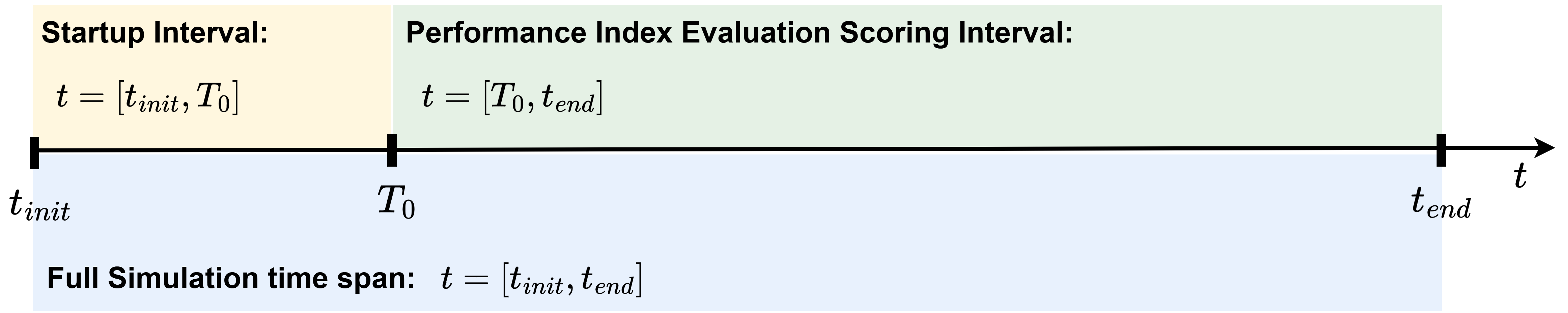
../_images/startup_int_vs_scoring_int.png — Figure 9 Key time intervals for performance evaluation.¶

Controller Definition¶

Important

Your control law (my_controller) must be defined for the entire simulation duration (\(t \ge 0\)), even though the performance index is computed only during the scoring interval.

Evaluation Criteria¶

Important

Performance Index (\(\mathcal{G}\)): evaluated during the scoring interval (\(t \ge T_0 = 30\) s).
Passivity constraint: \(p_{pto} \ge 0\) must hold for the full simulation.

See Evaluation Criteria & Competition Rules for a complete description.

Evaluation Mode — Controller Adaptation Requirement¶

During Evaluation Mode (eval_flag = true), the WAPPAC platform executes the three official sea-state scenarios (wave_id = 1–3) in a aleatory order. Controllers do not receive any prior information about which sea state is being simulated and should therefore adapt adequately to the prevailing conditions.

Participants are encouraged to verify controller robustness under unknown sea states by running equivalent randomized tests in development mode (eval_flag = false). This capability is essential for achieving a consistent and high performance index across all evaluation cases.

Startup Ramp¶

The wave excitation force is introduced smoothly through a raised-cosine ramp:

\[ramp(t) = 0.5 \left[ 1 - \cos\!\left(\frac{\pi t}{T_{ramp}}\right) \right]\]

where \(ramp(T_{ramp}=20)=1\). Refer to Numerical Implementation for further details.

Important

Ramp duration is fixed to \(\mathbf{T_{ramp}} = 20\) s for all simulations across the three sea states scenarios.

Control Update Scheme (Zero-Order Hold)¶

The control force is updated at the beginning of each simulation time step (\(\Delta t = 0.05\ \text{s}\)). Internally, the solver performs Runge–Kutta (RK4) sub-steps while holding the control force constant (Zero-Order Hold). See WavePiston Dynamics Numerical Integration for implementation details.

Numerical Limitations and Control Definition¶

The WAPPAC simulator provides a numerical approximation of a continuous-time physical system. Controllers that induce rapid or discontinuous dynamics, with response times close to or faster than the simulation timestep, may lead to numerically unstable or dynamically inconsistent behavior that no longer represents a physically meaningful response.

Important

The continuous system approximation breaks when control-induced changes occur close to or faster than the simulation timestep.

Rapid Dynamics Limitation¶

As a rule of thumb to maintain a physically meaningful simulation, the change in velocity caused by the applied PTO force over a single time step

\[ \Delta v \approx \frac{F_{\text{pto}},\Delta t}{M} \]

should remain small compared to the typical device velocity. If \(\Delta v\) becomes of the same order or larger than the typical velocity magnitude, the discrete update may overshoot or invert the motion direction within one step, leading to numerically inconsistent or unrealistic oscillatory behavior.

Example of Unrealistic Dynamics¶

A Coulomb-type control law with a very high gain (e.g. \(C_{pto} = 10^6\) N, the maximum allowed PTO force) causes fast changes in velocity within a single time step. This leads to unrealistic oscillations and unstable numerical behavior.

By experimenting with this configuration, participants can observe the effect directly:

def my_controller(x, v, t, eta10):
    # Example of overly stiff control (numerically unstable)
    C_pto = 1e6  # very high gain
    F_pto = C_pto * np.sign(v)
    return F_pto

To mitigate this behavior, one possible approach is to lower the control gain — for example:

def my_controller(x, v, t, eta10):
    # More moderate control gain (numerically stable)
    C_pto = 1e4
    F_pto = C_pto * np.sign(v)
    return F_pto

This adjustment preserves the intended Coulomb damping effect while ensuring a smoother numerical response.

Other alternatives participants may consider include:

Introducing a smoothed control law, for instance replacing the discontinuous sign function with a continuous approximation such as F_pto = C_pto * np.tanh(v / v_ref), where v_ref defines a small transition range.
Updating the control law at a slower rate (multiple \(\Delta t\) ZOH) to reduce abrupt changes between successive time steps.
Incorporating mild viscous damping or rate limiting in the force computation.

These strategies could help achieving consistent and more realistic dynamic responses while maintaining the intended overall control strategy. Participants must be aware of numerical limitations of the WAPPAC platform when designing their controllers.

Important Note on Evaluation Metrics¶

The mean absorbed power and performance index do not inherently penalize rapid or discontinuous variations in force or motion. As a result, controllers that inadvertently exploit numerical artifacts may achieve artificially high scores.

Participants are encouraged to check this effect using the Coulomb-like control example above with \(C_{pto} = 10^6\) N.

Important

Results exhibiting high performance by exploiting numerical artifacts or due to non-physical behavior will not be considered valid for evaluation.
Only simulations demonstrating stable, physically consistent dynamics will be accepted.

Handling Up-Wave Data (`eta10`)¶

The signal eta10 (10 m up-wave surface elevation) is available only during the scoring interval. For \(t < 30\) s, eta10 = NaN. Your controller must handle this robustly.

Example:

def my_controller(x, v, t, eta10):
    if not np.isnan(eta10):
        # Optional preview or estimation logic
        pass
    # Example: proportional-velocity control
    F_pto = 1e6 * v
    return F_pto

✅ Summary¶

Implement your control in a Python function named my_controller.
Ensure numerical stability and satisfaction of the passivity constraint (\(p_{pto} \ge 0\)) throughout the full simulation time span.
Use the provided inputs (x, v, t, eta10) for designing your control law.
External packages may be included via external_packages/ and a list of them submitted later as requirements.txt.
The controller should adapt effectively to the three sea-state scenarios simulated in aleatory order during evaluation mode.

Writing Your Controller¶

Controller Function Interface¶

Function Arguments¶

Function Output¶

Using External Packages¶

Installing a Custom Package Locally¶

Including Auxiliary Controller Modules¶

Allowed and Restricted Features¶

✅ Allowed¶

⚠️ Restricted (and why)¶

Key Controller Design Considerations¶

Controller Definition¶

Evaluation Criteria¶

Evaluation Mode — Controller Adaptation Requirement¶

Startup Ramp¶

Control Update Scheme (Zero-Order Hold)¶

Numerical Limitations and Control Definition¶

Rapid Dynamics Limitation¶

Example of Unrealistic Dynamics¶

Important Note on Evaluation Metrics¶

Handling Up-Wave Data (eta10)¶

✅ Summary¶

Handling Up-Wave Data (`eta10`)¶