Numerical Implementation
The model and control frameworks are implemented with a consistent numerical setup to ensure comparability across all control strategies submitted by participants. When developing your controller, the following implementation details should be carefully considered.
WavePiston Dynamics Numerical Integration
The WavePiston dynamics, given by (1), are integrated using a 4th-order Runge–Kutta (RK4) scheme.
The solver operates with a fixed time step of \(\Delta t = 0.05\) s.
Within each time step, RK4 performs four intermediate evaluations (stages) of the WavePiston dynamics function, modeled by (1), to estimate the state at the next time step:
Evaluates WavePiston dynamics once at the beginning of the time step, twice at intermediate points, and once at the end of the time step.
Excitation force: the excitation force is evaluated at each RK4 stage.
RK4 Implementation in PyTorch
The WAPPAC simulation platforms relies on PyTorch modified RK4 scheme transcribed below from the official documentation:
def rk4_alt_step_func(func, t0, dt, t1, y0, f0=None, perturb=False):
    """Smaller error with slightly more compute."""
    k1 = f0
    if k1 is None:
        k1 = func(t0, y0, perturb=Perturb.NEXT if perturb else Perturb.NONE)
    k2 = func(t0 + dt * _one_third, y0 + dt * k1 * _one_third)
    k3 = func(t0 + dt * _two_thirds, y0 + dt * (k2 - k1 * _one_third))
    k4 = func(t1, y0 + dt * (k1 - k2 + k3), perturb=Perturb.PREV if perturb else Perturb.NONE)
    return (k1 + 3 * (k2 + k3) + k4) * dt * 0.125
For interested readers, the official implementation can be reviewed in torchdiffeq library.
Control Update
The control force \(F_{pto}(t)\) is implemented using a zero-order hold (ZOH):
The controller is evaluated once at the start of each simulation time step (\(\Delta t\)).
During RK4 internal evaluations or stages, the control force is held constant.
Practically, this means your controller function
my_controlleris called once per time step of duration \(\Delta t\).
Numerical Representation Limitations
The WAPPAC simulator provides a numerical approximation of a continuous-time physical system. Controllers that induce rapid or discontinuous dynamics, with response times close to or faster than the simulation timestep, may lead to numerically unstable or dynamically inconsistent behavior that no longer represents a physically meaningful response.
Important
The continuous system approximation breaks when control-induced changes occur close to or faster than the simulation timestep.
Rapid Dynamics Limitation
As a rule of thumb to maintain a physically meaningful simulation, the change in velocity caused by the applied PTO force over a single time step
should remain small compared to the typical device velocity. If \(\Delta v\) becomes of the same order or larger than the typical velocity magnitude, the discrete update may overshoot or invert the motion direction within one step, leading to numerically inconsistent or unrealistic oscillatory behavior.
Consequences
Results showing unrealistic behavior due to numerical issues, will be carefully reviewed and may be excluded from evaluation.
Participants are encouraged to design controllers that avoid impulsive or discontinuous actions and ensure smooth, realistic device responses. Practical guidelines and examples are provided in Writing Your Controller.
Ramp Interval
To reduce large transients at the start of the simulation—which could induce sail position drift and premature constraint violations—the wave excitation force is gradually applied during the ramp interval, illustrated in Figure 8.
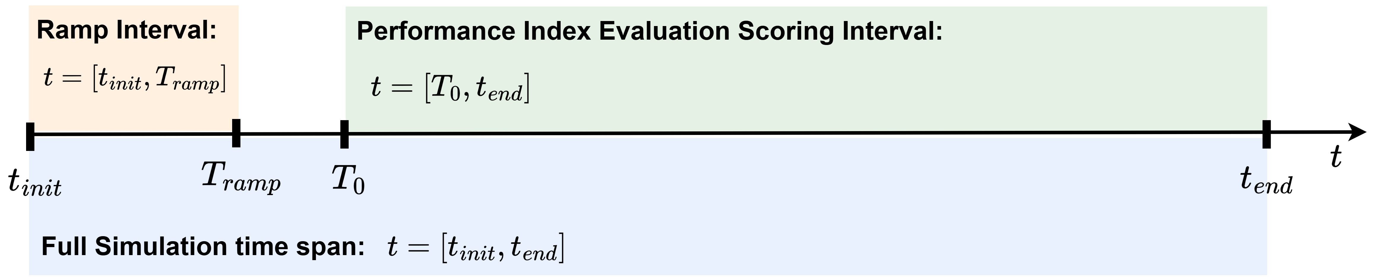
Figure 8 Ramp interval versus scoring interval.
The ramp function is defined as a raised cosine:
This function multiplies the excitation force from zero to its full value over the interval \(0 \le t \le T_{\text{ramp}}\). Thus, the attenuated excitation force is given by:
Note that the raised cosine time derivative is zero at both the start (\(t=0\)) and end \((t=T_{\text{ramp}})\) of the ramp, ensuring a smooth transition. Also, \(ramp(T_{\text{ramp}}) = 1\), so the excitation force reaches its full magnitude exactly at the end of the ramp interval.
Note
The ramp interval duration is fixed for every simulation at \(T_{\text{ramp}} = 20\) s across all three predefined sea state scenarios.
For \(t \ge T_{\text{ramp}}\) → \(\tilde{F}_{exc} = F_{exc}\).
The ramp interval ends before the scoring interval begins (\(T_{ramp}=20 < T_0 = 30\) s), mitigating transient effects of the artifical ramp-up function before start evaluating the performance index.
Up-wave Measurement
Linear wave theory is used for modeling the wave surface elevation, using a seawater depth of \(d=10000\) m (~ Inf), and density of \(\rho=1025\) \(\text{kg/}\text{m}^3\).
Handling Up-wave Measurement
Important
Up-wave measurement is available only during the scoring interval (\(t \ge T_0\)).
For \(t < T_0\), the measurement value is
NaN. Refer to Writing Your Controller for instructions on handlingNaNinputs safely in your control strategy.